Physics to the rescue

Fortunately free-field calibration is not the only method. There are couple of others. Well, maybe more then couple if we take into account metallic membranes that can be excited electronically. But let’s stick to acoustical excitation.

So there are different microphone types, depending on application sound field. They have to have straight frequency response when subjected to their corresponding sound field in which they were calibrated. Free-field mic presumes you will be measuring single sound source straight on it’s axis. This is what you want for speaker measurement. Diffused-field mic expects multiply random sound sources from all directions. This type of mic you would use to accurately record an event in a highly reverberant space (like church). In a case of pressure-field mic, only it’s membrane is subjected to a sound-field. So you would use it to measure sound pressure in a closed chamber or pressure at some boundary (like a baffle).

You wouldn’t use pressure-field calibrated microphone in a free-field speaker measurements and expect it to have full linear frequency response and vice versa.  But as you can see from the graph above, all those fields converge at lower frequencies. And it makes perfect sense (I hope). As microphone dimensions are getting smaller and smaller in comparison to excitation wavelengths, it’s no longer disturbing the sound field with its presence. We can use this to our advantage and construct a piston driven closed chamber with almost perfect pressure-field. Then, at the constant temperature,  the pressure in this chamber will solely depend on the volume displaced by the excitation piston.

Pressure is inversely proportional to the volume. That’s Boyle’s law and it’s physics 101. Now the thing to watch out for is the frequency at witch we are moving the piston. If we are moving it too fast – pressure-field will collapse and we will create standing waves. So we want our chamber longest dimension to be between 1/6 and 1/8 wavelength of the highest piston frequency.

If we choose our cut-off frequency to be 500Hz (or wavelength of 68cm), then our pressure chamber length should be between 11.5 and 8.6 cm. I’m oversimplifying this as much as I can. There is excellent app-note from Ivo Mateljan, creator of ARTA measuring software with more in-depth explanations and some math to back it up.

Practical realization

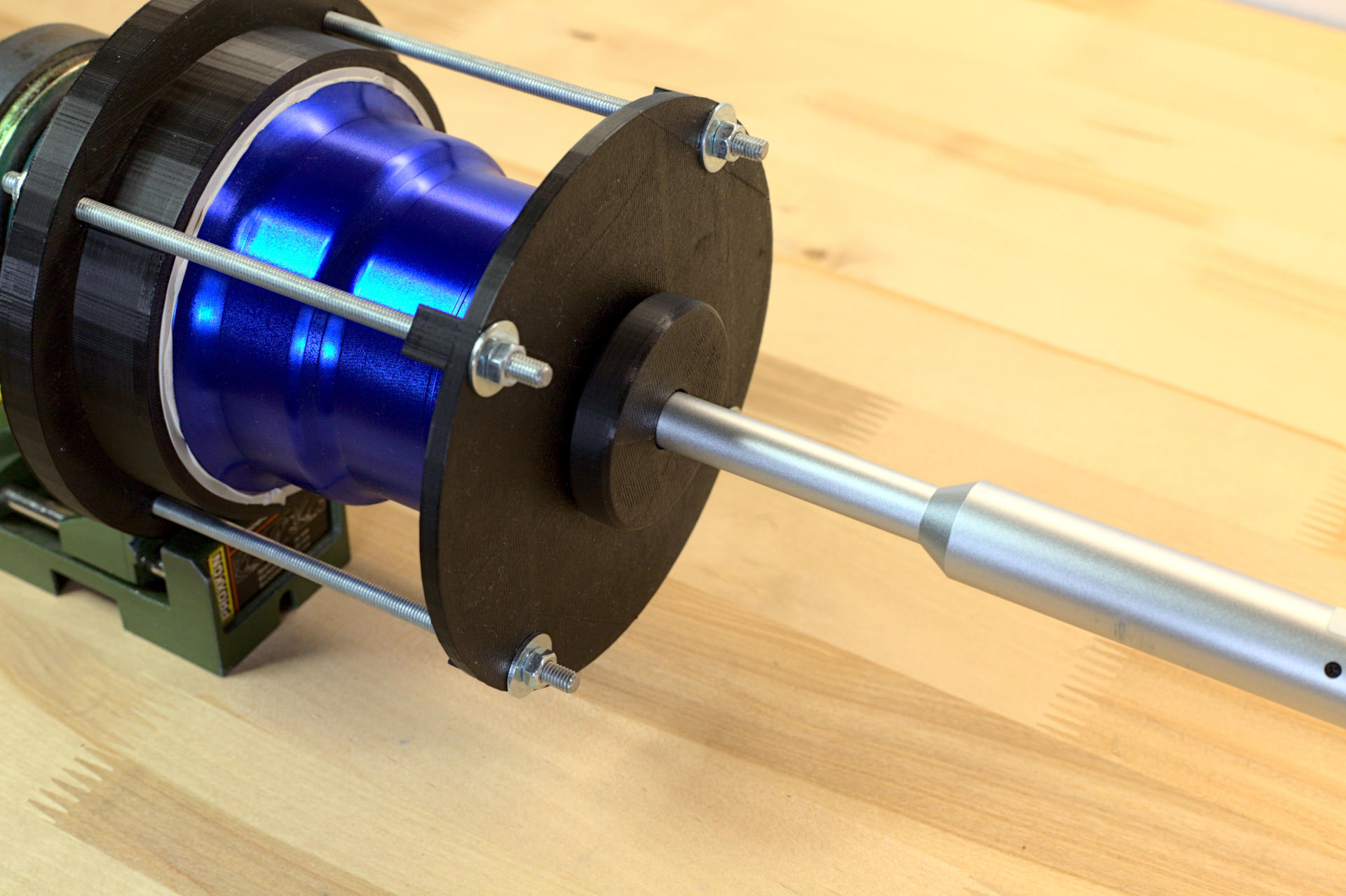
I didn’t found Visaton FRS8 for a sale locally and all the COVID-19 pandemic restrictions was just kicking in. Shipping was taking forever so I decided not to be lazy and use some other driver. It just so happens I had a modified DLS 424 cox driver without the tweeter (glued cap). It’s a 4″ mid driver that I was experimenting some long time ago. It’s no longer produced so I don’t see any point in publishing my exact pressure chamber design. Instead I redesigned it for a 3.3″ Visaton driver based on datasheet dimensions. So blame them if it doesn’t fit!

Use a regular 75mm OD PVC waste pipe for tube part. Or you can print it if you think that’s a good idea. It’s length should be 101mm, so you would get the same volume of 0.39L as in the app-note. There is a 3mm relief in both end-plates. Use a rubber seal or just some silicon hermetic to seal all parts and tighten them with 5mm rods.

The importance of driver parameters

In order to get a reliable mathematical model of the constructed pressure chamber we will need to know these parameters:

• Voltage level used to drive the excitation piston (driver).
• Total volume of the pressure chamber.
• Thiele-Small parameters of the driver.

We can measure voltage very accurately with a good multi-meter or calibrated sound-card. And we can calculate pressure chamber volume quite easily as πr²h. Plus small amount of driver membrane volume. In case of SFR8 it’s negligible, but on some other more conical drivers it can be substantial. So take that into account also.  And finally we need to know T/S parameters for the driver. That’s were biggest potential for uncertainty lies. I would not trust manufacturer datasheet values for a second. They are in a ball-park usually, but I yet have to measure a driver were they agree 100%. So even if using SFR8 driver I urge you to measure it yourself. It’s quite trivial measurement with a free software like REW. Use 5g of modeling clay on dust cap for added weight and make sure you calibrated your sound card for impedance measurement.

You’ll have to input voice coil DC resistance which again is an easy multimeter measurement and membrane area Sd. Later could be more tricky to calculate. But you can just decompose it to couple simple geometrical figures.

Cone is just a conical frustum and cap is just a… well, cap. Measure the relative surfaces and use any online calculators to solve for surface area. Suspension is kinda grey area. It will depend on its construction as to how much of it will actually “play”. But solving for half of torus surface area and then taking 30% will bring you into the ballpark.

To get a good idea of how reliable your measured T/S parameters are, we can do a cross-check. Just plug your T/S data to any box simulation software (like free WinISD), select closed box with a volume equal to your chamber and simulate the resulting driver impedance. Then measure the real driver impedance with a sealed chamber and check how well the resonance frequencies match. As you can see above, mine were within one Hertz.

Mathematical model

I didn’t try to reinvent the wheel and just used a MatLab script from the app-note. You can download it here. I increased calculation points to 500 for better definition. MatLab is available as a 30 day trail (for free), so there are no problems running this script as an one off experiment.

Above are MatLab generated SPL graph for my pressure chamber. With a standard 2.83Vrms input we can expect some 150dB of pressure inside it! That’s close to a rocket launch sound levels, so you wouldn’t want to put your head inside it. Or your microphone for that matter. Instead I used voltage of just 10mVrms. That way at the frequency of 300Hz I get 94dB. Very convenient for future mic sensitivity evaluation.

MatLab generated resonance frequency is again, basically spot-on measured one. This gives me high confidence level in overall experiment accuracy.

I didn’t found a straight-forward way to export MatLab variable values. So I just opened variables f (frequency) and pudb (SPL inside the box), transposed them horizontally and copied to excel. Then saved file as comma-delimited for further import to measurement software.

Calibration

Now that we have a theoretical pressure chamber SPL data, it can be used as a reference for comparison to SPL data measured with a microphone. The difference between the two will be a microphone calibration curve. Ideally we would want to first measure it with some reference microphone and make sure theory complies with reality. But I don’t think many of us has such $$$$ mic laying around “just in case”. So if one was meticulous enough and did all the cross-checks mentioned above – there should be nothing to worry about.

First lets start with measurement setup calibration. We want to be sure, that all the low-frequency roll-off of a sound card and amplifier are accounted for. This is really critical, otherwise results will be inaccurate. I’ll try to walk you through, so the next chapters will be more “how to” then just results. I will be using REW for this example so calibration procedure is documented here. I will just add that it’s really preferable to use ASIO interface and avoid any mixer nonsense. When done correctly – you  expect to see a straight line for a measurement setup as pictured above.  Next let’s level calibrate the rig.

Connect multimeter to driver terminals, open REW generator and set it to sine-wave and -6dB level. Adjust amplifier level so that multimeter will show 1Vrms. Open REW SPL meter and press “Calibrate”, enter 0 and press “Finished”. Now press “Measure”, set level to same -6dB and press “Start Measuring”.

If everything was done correctly – you will end up with a graph like above. That means you are now level and frequency calibrated and 0dB is in fact 1Vrms or 0dBV in short. Now let’s set output level to 10mV. To do so, we need to lower level 100 times or 40dB, so we lower generator level from -6dB to -46dB. Check that you measure ~10mV. At this point we can start to introduce a microphone to the system.

I made a rubber shim to seal the microphone in a chamber. Modeling clay works too but it’s more messy. I will not repeat the findings of app-note figure 10, regarding the importance of total air tightness. It’s really critical for the lowest octave.

Don’t forget to set the measurement level to -46dB! As -6dB will definitely destroy your mic. Now connect your microphone straight to sound card input. You can use this phantom power unbalancing circuit if your sound card doesn’t have balanced inputs.

Select R_in such, that resulting R_total would be equal to your pre-amp (or whatever you will be using) input impedance. Don’t forget to account for your sound card input impedance R_s . The main idea here is that you know the exact impedance that mic is working into for a proper sensitivity estimation.  Another thing to watch out is your mic output type. If it’s fully-balanced (there is inverse signal on Pin3) – you have to add +6dB to your measurement. That is if you’re planning using it with balanced input. Now hit “Start Measure” and listen to the sweep.

Above are my measurements for EMM-6 (red) and WM61A (blue) mics. There is no smoothing (or any other post-processing applied). If you have sharp peaks or valleys in your graph – something went really wrong. Review your setup and find what that was.

Extracting the information

The good news is that we already know the absolute sensitivity of our mics!  As can be seen from MatLab SPL simulation – that’s a point in graph at 300Hz.

So for EMM-6 mic that would be -42.66dBV or 7.35mV/Pa. Here is explanation how we made a mental leap from 94dB to Pascals (in case you were wondering). With a little bit of faith (that our mic is linear from 300Hz to 1kHz) we can state that it’s absolute sensitivity is 7.35mV/Pa@1kHz in to 1kΩ (my total setup impedance). This assumption is not far from truth as we will soon see.

Above are absolute sensitivity table of my measurement microphones. I also measured pressure-chamber with my SPL meter at single 300Hz frequency. Then I added A weighting correction of +7.09dB and got 94.8dB. Which is +0.8dB over of what it should measure. I firmly believe that it’s an error of this cheap ±1.5dB device and not my measuring setup.

We’ll have to work a little bit more to extract our calibration curves. First open saved MatLab SPL file and extend it to 2Hz (copy same SPL value as 10Hz). Then import this measurement to REW and add negative offset. This offset should be equal to difference @300Hz between your MatLab and measured SPL’s. In my case its 94dB+42.66dB=136.66dB. The idea here is to have a good match @300Hz. You should end-up with something like this:

Now open Controls, select your measured SPL for trace A and MatLab generated for trace B, choose A/B arithmetic function and press generate.

And voilà – you have your microphone calibration curve. It’s should be valid up to 300Hz. Then microphone positioning inside the chamber starts to have a noticeable influence.  Again, my findings is well in accordance with app-note figure 9 on this matter.

And finally – here are my full calibration curves. They’re merged with my reference 1″ dome baffle measurement @300Hz. So 300Hz-1kHz region is subjected to some interpretation, but it’s under 0.5dB of potential error. So I’m not planning to lose my sleep over it.